- Employment Surveys
Collection of U.S. unemployment statistics began during World War II to identify areas where labor market imbalance was created as a result of an inadequate labor supply, materials shortages, and transportation difficulties. After the war, emphasis was placed on identifying areas of labor surplus (high unemployment).
Labor force and unemployment statistics are obtained from the Current Population Survey (CPS). The CPS is a monthly survey, conducted by the Bureau of the Census, of about 50,000 households representing the civilian noninstitutional population. Respondents are interviewed to obtain information about the employment status of each member of the household 16 years of age and over. Each person is classified into one of three categories based on their status during the calendar week, Sunday through Saturday, which includes the 12th day of the month (the "reference week"):
- Employed
- Unemployed
- Not in the work force
The CPS provides comprehensive data on the labor force, the employed, and the unemployed, classified by such characteristics as age, sex, race, family relationship, marital status, occupation, and industry attachment. The survey also provides data on the characteristics and past work experience of those not in the labor force.

Figure 6-1. Average annual U.S. unemployment rates. Data Source: U.S. Dept. of Labor, Bureau of Labor Statistics (http://www.bls.gov/)
Additional unemployment data is obtained from state unemployment insurance programs and the monthly Current Employment Statistics (CES) Survey. The CES survey is designed to provide industry information on nonfarm wage and salary employment, average weekly hours, average hourly earnings, and average weekly earnings. The employment, hours, and earnings data are based on payroll reports from a sample of over 390,000 establishments employing over 47 million nonfarm wage and salary workers.
Civilian Noninstitutional Population - persons 16 years of age and older who are not inmates of institutions (e.g., penal and mental facilities, homes for the aged) and who are not on active duty in the Armed Forces.
Employed Persons - persons 16 years and over in the civilian noninstitutional population who, during the reference week, (a) did any work at all (at least 1 hour) as paid employees, worked in their own business, profession, or on their own farm, or worked 15 hours or more as unpaid workers in an enterprise operated by a member of the family, and (b) all those who were not working but who had jobs or businesses from which they were temporarily absent because of vacation, illness, bad weather, childcare problems, maternity or paternity leave, labor-management dispute, job training, or other family or personal reasons, whether or not they were paid for the time off or were seeking other jobs. Each employed person is counted only once, even if he or she holds more than one job. Excluded are persons whose only activity consisted of work around their own house (painting, repairing, or own home housework) or volunteer work for religious, charitable, and other organizations.
Unemployed Persons - persons 16 years and over who had no employment during the reference week, were available for work, except for temporary illness, and had made specific efforts to find employment sometime during the 4-week period ending with the reference week. Persons who were waiting to be recalled to a job from which they had been laid off need not have been looking for work to be classified as unemployed.
Labor Force - Total employed + total unemployed.
Unemployment Rate - The total number unemployed as a percentage of the labor force.
Unemployment Rate = (Number Unemployed / Labor Force) * 100
Not in the Labor Force - All persons in the civilian noninstitutional population who are neither employed nor unemployed. Information is collected on their desire for and availability to take a job, job search activity in the prior year, and reason for not looking in the 4 week period prior to the survey week. This group includes discouraged workers, defined as persons not in the labor force who want and are available for a job and who have looked for work sometime in the past 12 months, but are not currently looking because they believe there are no jobs available or there are none for which they would qualify.
Participation Rate - The labor force as a percentage of the civilian noninstitutional population.
     Participation Rate =             Labor Force              * 100
                          Civilian Noninstitutional Population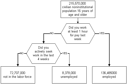
Figure 6-2. U.S. Labor Force: Employment, Unemployment, and Unemployment Rate, 2002.
Data Source: U.S. Dept. of Labor, Bureau of Labor Statistics (http://www.bls.gov/)2002 Total labor force = 8,378,000 + 136,485,000 = 144,863,000
2002 Participation rate = ( 144,863,000 / 217,570,000 ) * 100 = 66.6%
2002 Unemployment rate = ( 8,378,000 / 144,863,000 ) * 100 = 5.8%The share of the population participating in the labor force (participation rate) is an important statistic when examining unemployment over time and across countries. For example, the participation rate of women in the U.S. labor force has increased dramatically over the last three decades, while the participation rate of men has declined slightly.

Figure 6-3. Average annual U.S. labor force participation rates by gender. Data Source: U.S. Dept. of Labor, Bureau of Labor Statistics (http://www.bls.gov/)
- Demographics of Unemployment
The unemployment rate can vary widely between demographic groups. Unemployment tends to be greater among minorities (Figure 6-4), females (Figure 6-5), and teenagers (Figure 6-6). In addition, unemployment is generally lower for skilled workers and college graduates.

Figure 6-4. Average annual U.S. unemployment rates by race. Data Source: U.S. Dept. of Labor, Bureau of Labor Statistics (http://www.bls.gov/)

Figure 6-5. Average annual U.S. unemployment rates by gender. Data Source: U.S. Dept. of Labor, Bureau of Labor Statistics (http://www.bls.gov/)

Figure 6-6. Average annual U.S. unemployment rates by age. Data Source: U.S. Dept. of Labor, Bureau of Labor Statistics (http://www.bls.gov/)
The difference in unemployment rates between males and females does have some interesting twists. First, the labor survey has not been completely unbiased. When the survey was started the "Are you working?" question was put differently to men and women. Men were asked, "Last week, did you do any work for pay or profit?" Women were asked, "What were you doing last week, keeping house or something else?" Women who may have been looking for work may still have answered, "keeping house," and were not counted as unemployed. It wasn't until 1994 that the labor survey was changed to ask men and women the same question.
Second, the difference in unemployment rates between men and women was the greatest from the early 1960s to the late 1970s. This period corresponds to the dramatic growth in the labor force participation rate by women shown in Figure 6-3. New entrants to the labor force have a higher unemployment rate and this shows up in the gender gap.
- Criticisms of the Unemployment Rate
Unfortunately the unemployment rate is not a perfect indicator of economic activity or inactivity. There are three areas of criticisms regarding the measurement of the unemployment rate:
1. Survey accuracy.
2. Discouraged workers
3. Underemployed workersFirst, all surveys are subject to difficulties that may affect survey accuracy. For example, telephone surveys will exclude people who don't have phones. If the unemployed are more likely not to have phone service then the unemployment rate could be understated. Perhaps a greater problem is that to be counted as unemployed the individual being surveyed must admit that he or she is out of work. This is embarrassing and can motivate a person to lie. Offsetting this tendency to understate the unemployment rate are survey respondents who say they are actively looking for work when they are not. For example, individuals who are receiving unemployment benefits or other income assistance must report they are actively seeking work to keep getting benefits. These persons may say they are looking for a job when they actually are not. Survey organizations must invest great effort to minimize or correct for these possible survey distortions.
Second, the unemployment rate only counts those who are actively looking for work. It does not count those who would like to work but have given up finding suitable employment. The CPS was redesigned in 1994 to include a separate category for discouraged workers. Discouraged workers are those who would like a job, have looked for work in the last 12 months, are available for work, but are not currently looking for work because they don't believe they can find anything suitable for their skills, don't have the necessary skills or training, are too young or too old, or have faced other forms of discrimination. Discouraged workers are not counted as part of the labor force and are not counted as unemployed. Consequently, the unemployment rate may understate actual unemployment.
Discouraged workers are of interest because they, like the unemployed, represent unused human resources in the economy. Table 6-1 shows that an average of 4.68 million persons reported that they would like to work in 2002, representing about 6.4 percent of all persons outside the labor force. If these discouraged workers counted as unemployed the average 2002 unemployment rate would have increased from 5.8 to as much as 9.0 percent
Table 6-1. Discouraged Workers (thousand of persons, annual averages) 2000 2001 2002 Total not in the labor force 69,994 71,359 72,707 Persons who currently want a job 4,413 4,590 4,677 Searched for work and available for work now (1) 1,157 1,266 1,439 Reason for not looking: Discouragement over job prospects (2) 262 321 369 Reasons other than discouragement (3) 895 945 1,070 (1) persons who have searched for work during the prior 12 months and were available to take a job during the reference week.
(2) includes thinks no work available, could not find work, lacks schooling or training, employer thinks too young or old, and other types of discrimination.
(3) includes those who did not actively look for work in the prior 4 weeks for such reasons as child-care and transportation problems, as well as a small number for which reason non-participation was not determined.
Source: Bureau of Labor Statistics, U.S. Department of Labor (http://www.bls.gov)A third problem with the unemployment rate as a measure of overall labor activity is that the employed may not be working as much as they would like. The underemployed may be working part-time but would prefer a full-time job, may be employed full-time but working at less than capacity, or may be overqualified for their current positions. For example, Figure 6-7 shows that the average hours worked per week in manufacturing generally declines during recessions. Again, the unemployment rate alone may understate actual unemployment or the slack in the economy.
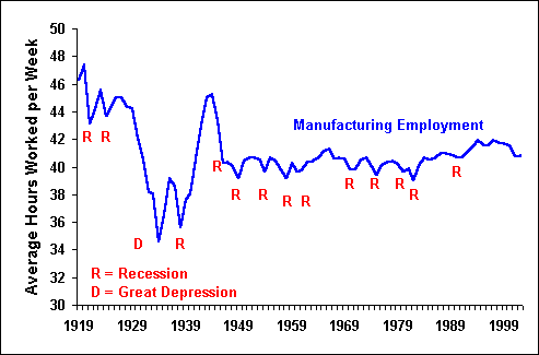
Figure 6-7. Average Hours Worked per Week in Manufacturing.
Discouraged Workers - persons not in the labor force who want and are available for a job and who have looked for work sometime in the past 12 months, but who are not currently looking because they believe there are no jobs available or there are none for which they would qualify.
Underemployment - persons in the labor who are working but are not working all the hours they are willing and able to.
Unemployment may be characterized according to its causes. We generally classify unemployment into four basic types:
- Frictional Unemployment
- Structural Unemployment
- Seasonal Unemployment
- Cyclical Unemployment
Frictional Unemployment is associated with a dynamic labor force in a stable economy with imperfect information about available jobs. People are just entering the labor force or moving between careers and locations (dynamic labor force) and while there are job openings (stable economy) it takes time to find a new job (imperfect information). We should expect with the Internet as a growing new source of job information that job search time and frictional unemployment should decline. However, the process of applying and interviewing for a new job remains costly in terms of time required.
Structural Unemployment is associated with a stable labor force in a dynamic economy. There may exist a mismatch between workers' skills and the skills required for available jobs. For example, as technology progresses new industries arise and mature ones decline. Badly managed firms go bankrupt and new firms are formed. Structural unemployment results when the location and/or skills of the labor force do not match the available jobs. It takes time for displaced workers in one region of the country to find comparable work elsewhere, or receive retraining for the skills required with different or new technologies.
Seasonal unemployment is associated with the seasons of the year. Some businesses and industries experience a peak in consumer demand during the last half of the year leading up to Christmas. Snow skiing and Florida beach resorts are busiest during the winter. Many other resorts have customers only during the summer.
The published unemployment statistics are often reported as "seasonally adjusted" numbers in order to eliminate the normal seasonal changes. For example, if the unemployment rate increases from 5 percent in December to 5.5 percent one month later in January, should we be surprised and suspect the economy is slipping into a recession? Probably not, especially if we normally see such increases in the unemployment rate from December to January. The seasonally adjusted unemployment rate provides a measure that lets us more easily recognize unusual or unexpected month-to-month changes.
Seasonal adjustment essentially asks the question, if we have a 5.5 percent unemployment rate in January, what would we expect the annual average unemployment rate will be? Consider the trend in unemployment for 2001 as shown in Table 6-2. From January to December the raw (unadjusted) unemployment rate increased from 4.7 percent to 5.4 percent. That does not appear to be a particularly large increase. The seasonally adjusted numbers, however, reveal a more dramatic increase, from 4.2 to 5.8 percent. A 4.7 percent January unemployment rate is usually consistent with an annual average unemployment rate of 4.2 percent. The 5.4 percent December unemployment rate is usually consistent with an annual average unemployment rate of 5.8 percent.
| Table 6-2. Unadjusted Versus Seasonally Adjusted Unemployment Rates | ||
| (percent)) | ||
| Month | Not Seasonally Adjusted |
Seasonally Adjusted |
| January, 2001 | 4.7 | 4.2 |
| February | 4.6 | 4.2 |
| March | 4.6 | 4.3 |
| April | 4.2 | 4.5 |
| May | 4.1 | 4.4 |
| June | 4.7 | 4.6 |
| July | 4.7 | 4.6 |
| August | 4.9 | 4.9 |
| September | 4.7 | 5.0 |
| October | 5.0 | 5.4 |
| November | 5.3 | 5.6 |
| December, 2001 | 5.4 | 5.8 |
| Source: Bureau of Labor Statistics, U.S. Department of Labor (http://www.bls.gov) | ||
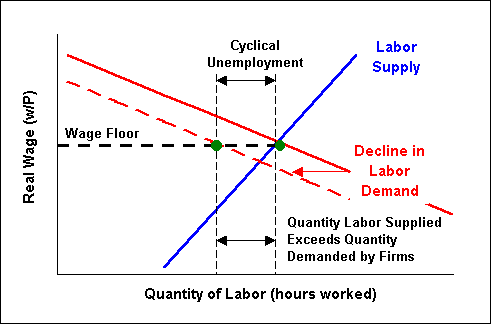
Cyclical Unemployment is associated with business cycles and, more particularly, with temporary downturns in the economy. During recessions the demand for products and services declines, workers are laid off, and (cyclical) unemployment increases. The demand for labor is derived from the demand for goods and services. When the demand for goods and services declines then the demand for labor drops as well.
Frictional Unemployment - unemployment that results from people entering the labor force or voluntarily moving between careers or locations. Information about available jobs and available workers is imperfect and therefore job search takes time. Structural Unemployment - unemployment that results from a mismatch between workers' skills and the skills required for available jobs. Seasonal Unemployment - unemployment that results from the normal seasonal change in aggregate economic activity. Cyclical Unemployment - unemployment that results from a decline in aggregate economic activity that occurs during business cycle contractions (e.g., recessions). |
You should recognize that we have not really drawn sharp distinctions between these types of unemployment. A worker may quit one job because it is in a declining industry to look for a better job in a growing industry. Is this frictional or structural unemployment? We suggested that new entrants into the labor force represented frictional unemployment, but during recessions it becomes much harder for new entrants to find jobs. Is this frictional or cyclical unemployment?
What is important to realize is that there will always be some level of unemployment that no force in heaven or in Congress can eliminate. Frictional, structural, and seasonal unemployment are three types of unemployment that always exist in an economy and thus prevent the unemployment rate from ever reaching zero.
Cyclical unemployment is generally considered the most important and the one on which our macroeconomic models are focused. Congress may act aggressively to stimulate the economy during recessions and lower cyclical unemployment such as through tax cuts or increased government spending. This will be a primary topic of following chapters in this course.
Full employment represents the complete utilization of available resources. At full employment an economy would be on its production possibilities frontier. But, because of the existence of frictional, structural, and seasonal unemployment, an economy's unemployment rate is never zero, even when the economy is at its "full-employment" level. The rate of unemployment that prevails when the economy is at its full-employment level of output is called the natural rate of unemployment.
It is very difficult to say exactly what the natural rate of unemployment is. During the 1950s, most economists believed the natural rate was in the 4 to 5 percent range. The natural rate grew to about 6 percent in the 1970s because of the surge of teenagers from the baby boom generation entering the labor market, and has fallen back to less than 5 percent in the 1990s (if you are unfamiliar with the term "baby boom" let's just say that the men and women who returned home from World War II caught up on unfinished business, which significantly impacted the labor market some 16 years and 9 months later). The reason for changes in frictional and structural unemployment rates over time include changing demographics as mentioned above and changes in minimum wages, racial and sex discrimination, and unemployment benefits among other factors.
Because frictional and structural unemployment cannot be directly measured, the natural rate of unemployment is a theoretical concept that is often defined as the rate at which increases in aggregate demand for output lead mostly to higher prices and wages rather than output and employment. In other words, let's say the economy is at full employment output and unemployment is at the natural rate. Experienced available labor becomes hard to find. If there is an increase in demand for products and services then firms will start to raid labor from other firms by offering higher wages. When paying higher wages firms must increase the price of their product or service. The result is no actual increase in the level of employment or total output but an increase in prices. But we do not have the situation in a microeconomic supply-demand model where an increase in price reduces the quantity demanded. In a macroeconomic model there may be no reason to expect a reduction in demand because wages are rising at the same rate as prices. Therefore, as long as demand remains above the level that can be satisfied at full employment output we can have a sustained period of rising prices, i.e., high inflation.
Full Employment Output - the level of output at which the labor market is at its natural rate of unemployment. Natural Rate of Unemployment - unemployment arising from frictional, structural, and seasonal unemployment. Also described as the unemployment rate that coexists with macroeconomic stability. |
Full employment output is also described as the maximum sustainable level of output. Over short periods the economy could be operating above this level and at times below this level. As output fluctuates around the full-employment level of output during a business cycle, the unemployment rate fluctuates around the natural rate. When the economy is in a recession and output is below full employment output, cyclical unemployment is positive. During the inflationary peak of a business cycle, output could be above the full-employment level and cyclical unemployment is negative.
While the focus of this course is on the impact government can have on cyclical unemployment, government policy can also influence on the rates of frictional or structural unemployment. For example, the monthly government reports on regional unemployment rates can help workers identify the areas of the country where labor is most needed and make job search more efficient. Publicly funded retraining programs are designed to help workers transition from one industry to another. Such programs hopefully reduce the time needed to find new jobs and thereby lower the frictional and structural unemployment rates.
The government policy that is perhaps the most controversial with respect to its effect on structural and cyclical unemployment is unemployment insurance. Workers who are forced to leave their jobs through no fault of their own can collect a fraction of their wages for a certain period after losing their jobs. A typical unemployed worker can receive 50 percent of his or her former wages for 26 weeks. During recessions the government may extend the coverage period because of the greater difficulty in finding new jobs. Workers who voluntarily quit their jobs or who are fired for cause do not qualify.
Unemployment benefits certainly reduce the hardship to the individual from being laid off, but they also raise the level of the natural rate of unemployment. Those who receive unemployment benefits may feel less pressure to find a new job. With the unemployment compensation cushion they may turn down some job offers while waiting for something better. Cross-section studies that compare unemployment rates across regions of the country or between different countries generally find that those with more generous unemployment compensation benefits have higher unemployment rates. This is one of many examples we will run across where what is good for the individual may not produce the most desirable measure of aggregate economic performance.
