
 |
Intermediate Macroeconomics | |
6. The Neoclassical IS-LM Model |
The introduction of the Keynesian model in the 1930s represented a significant innovation in the way economists and policy-makers thought about the macroeconomy. Fiscal policy in the form of changes in government spending or taxes was seen as playing a pivotal role in managing economic growth and the economy. This didn't sit that well with the "classical" economists who still believed in small government and laissez faire.
By the 1940s the very strict Keynesian assumptions of sticky interest rates and prices presented a real problem. Once the economy was out of the Great Depression these assumptions just didn't hold. The foundation of the Keynesian model was extended to include variable interest rates and prices (beginning with Nobel laureate Sir John Hicks, "Mr. Keynes and the Classics: A Suggested Interpretation," Econometrics, April 1937). The Keynesian model became a special case of this more general model as we will show later in this chapter. This development also provided a second wind to the classical economists who used the model to show how active fiscal policy could be ineffective in stimulating the economy.
When we introduce variable interest rates we have to expand the method for solving the Keynesian macroeconomic model that we presented in the last chapter. In the Keynesian model we had one equation (aggregate expenditures) and one unknown (national income) and it was possible to solve for national income. If we add the interest rate as a new unknown variable we now have two unknowns so we must add at least an additional equation to solve the model. We do this by adding the monetary sector to our economy. Interest rates are determined by an equilibrium between money supply and money demand. This interest rate then influences aggregate expenditures and income. But it's not that simple. Aggregate expenditures and income also influence money demand so there are feedback effects. Nevertheless it is still easy to set up and simultaneously solve for the equilibrium income and interest rate.
The model we cover in this chapter is called the IS-LM model. The model is set up in two parts. First, the IS sector covers aggregate expenditures. The IS sector is identical to the Keynesian aggregate expenditures model presented in the last chapter with the exception that investment is now a function of the interest rate. Second, we add the LM sector, which includes money supply and money demand. Money demand is also a function of the interest rate as well as income. Finally, the two sectors are combined and solved simultaneously for equilibrium income and the interest rate.
You might have noticed that we haven't said much about prices. The average price level really plays no role in the model we develop in this chapter. Except for the period of high inflation of the 1970s this is generally not a problem (remember Occam's razor). We can add prices as a third unknown variable if we also add a third equation or market sector to solve the model. We could do that by adding a full-employment constraint, labor supply and demand (i.e., aggregate supply), or a Phillips curve but we should leave that for a later day.
![]()
The IS-LM model describes a macroeconomy with variable income and interest rates using two equilibrium relationships. The first relationship, the IS curve, focuses on the "goods" market (aggregate expenditures). The "IS" refers to the equilibrium relationship between investment and savings, although we will not present the model in these terms. In the simplest formulation of the model the interest rate affects only investment spending but can be extended to include household consumption with similar results. Because a higher interest rate reduces expenditures it also reduces income. Thus there is a negative relation between the interest rate and national income.
The second relationship involves the money market. The quantity of money demanded increases with income and decreases with the interest rate. An equilibrium in the money market occurs when the quantity of money demanded equals the quantity of money supplied. The points of all possible equilibria between money demand and a given supply of money is represented by the LM curve. If money demand is higher or lower than money supply then income and the interest rate must adjust to return the money market to equilibrium. An increase in income increases the demand for money (to conduct transactions). An increase in the interest rate is then needed to lower money demand back to the level of money supply. The "LM" refers to the traditional identification of money demand (L) and money supply (M) in money demand and supply graphs. Equilibrium occurs where the money demand curve (L) crosses the money supply curve (M).
The IS and LM curves are shown in Figure 6-1. The intersection represents the combination of interest rate and income where both the goods market (IS sector) and money market (LM sector) are each in equilibrium. An increase in government spending or a cut in taxes shifts the IS curve to the right, which raises both income and the interest rate. The magnitudes of the changes depend on the slopes of the curves and how far the IS curve shifts with a change in government fiscal policy. Keynesians suggest large income and small or no interest rate changes. Classical economists would argue there would be small income and large interest rate changes.
What is new in this model is that a change to money supply can also have an impact. An increase in money supply shifts the LM curve to the right, which increases income and lowers the interest rate. Again the magnitude of the changes depends on the slopes and size of the shift. Keynesians come down on the side of small income and small interest rate changes.
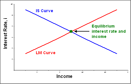
You might notice there is the interesting combination of fiscal and monetary policy changes. An increase in government spending (IS curve shifts right) combined with an increase in money supply (LM curve shifts right) can increase output without changing the interest rate. This is referred to as "accommodating" monetary policy. But here we run into the little problem with our assumption of a constant price level. Increases in both spending and money supply are likely to lead to higher prices. The IS-LM model is very useful...within its limitations.
Many of the debates between the Keynesians and Classical economists boil down to the values of the parameters in the underlying model equations. While the truth is always between the two extremes we won't try to pick the winners and losers here. For example, is investment sensitive to interest rates? It depends. Is the economy at the peak or trough of the business cycle? What is the relationship between short-term or long-term interest rates? The devil is always in the details. Our model will let us describe in general how an economy may react to changes in fiscal and monetary policy but it would take some sweat to quantify how much.
![]()
As we mentioned above, the IS curve represents all points of possible equilibria in the goods market. Generally, the setup of the IS curve is identical to that of the Keynesian model in the previous chapter, but with the interest rate added. We introduce variable interest rates to our model through investment. The revised investment equation is inserted into the accounting expression for aggregate expenditures (AE = C + I + G + NX). The IS equation is derived by applying the goods market equilibrium condition that national income equals aggregate expenditures (Y = AE) just like the Keynesian model. We finish this section by considering the characteristics of the IS equation that contribute to effective or ineffective government fiscal policy.
Investment is now assumed to be a negative function of the real interest rate. As the real interest rate increases, investment declines. Intuitively this should be obvious. A higher interest rate means it is more expensive to borrow money for capital investment. Some new capital investment that would have been made at low interest rates will not be made at high interest rates. (We discuss the relationship between investment and interest rates in more detail in a later chapter).
The investment function is presented in equation (1) and graphed in Figure 6-2. The investment curve slopes downward because an increase in the real interest rate makes investment more expensive and reduces the desired level of investment.
| I = I0 - b • i | (1) |
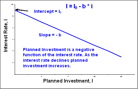
We start with the simple and hopefully familiar representations for aggregate expenditures. The only thing new is that investment is now a function of the interest rate as explained in equation (1) above.
Given:
AE = C + I + G + NX C = C0 + c • YD
|
Solving these equations using a procedure identical to that in the previous chapter on the Keynesian model (see Appendix A in this chapter for details of the derivation) yields equation (2), which represents the IS curve (Figure 6-3).
| iIS = 1 • (C0 + I0 + G0 - c • T0 + c • TR) - 1 - c(1-t) • Y b b |
(2) |
From equation (2) it is easy to identify the intercept and slope of the IS curve:
| IS curve intercept = | 1 • (C0 + I0 + G0 - c • T0 + c • TR) > 0 b |
| IS curve slope = | - 1 - c(1-t) < 0 b |
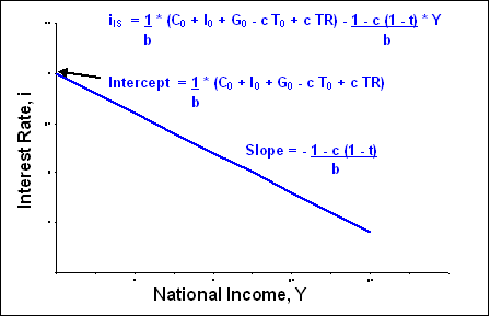
This basic version of the IS sector assumes a closed economy. There are no exports and no imports. Actually our assumption is that net exports (exports minus imports) equal zero, which is somewhat less severe. Assuming net exports equal zero simply suggests that imports and exports are insensitive to changes in either income or interest rates. The IS-LM model can be extended to allow for foreign trade but our results are not significantly affected. Such an extension would allow us to consider the effect of fiscal and monetary policy on the balance of trade, but we are more interested in this chapter is establishing the basic analytical method rather than exploring all permutations of the model.
The IS curve will shift to the left or right whenever the intercept of the IS curve changes. A change in any of the spending or tax variables in the intercept of the IS curve will cause the curve to shift. Any change in autonomous spending (C0, I0, or G0), lump sum taxes (T0), or government transfer payments (TR) will cause the IS curve to shift to the right or left. We can simplify our concerns by saying that any change in government fiscal policy (spending, taxes, or transfer payments) will cause the IS curve to shift.
| IS curve intercept = | 1 • (C0 + I0 + G0 - c • T0 + c • TR) > 0 b |
While the shift in the IS curve is technically up or down (the intercept becomes larger or smaller) we traditionally describe the shift as right or left. An upward shift in the IS curve is the same as a rightward shift. So, an increase in spending raises the value of the intercept of the IS curve, which causes the IS curve to shift upwards or, equivalently, to the right.
How much the IS curve shifts to the right depends on the size of 1/b. If 1/b is large (i.e., b is small) then a change in government fiscal policy leads to a larger shift in the IS curve. For example, an increase in government spending increases the interest rate. But because investment is insensitive to changes in the interest rate (b is small) there is little reduction in desired investment. In other words, an increase in government spending does not "crowd out" investment spending when the response of investment to changes in the interest rate, the b coefficient, is small. The greater the shift in the IS curve for a given change in government fiscal policy, the larger the potential change in income.
Note: we don't usually talk about a "change" in b, since the coefficient is assumed to be constant. We only talk about whether b is "large" or "small". Is investment sensitive (b is large) or insensitive (b is small) to changes in the interest rate?
The slope of the IS curve may be flat or steep again depending on the sensitivity of investment to the interest rate (i.e., the value of b).
| IS curve slope = | - 1 - c(1-t) < 0 b |
The IS curve is steep (slope is a large negative number) when investment is insensitive to changes in the interest rate (b is small). For a given change in the interest rate there is only a small change in investment and income.
The IS curve is flat (slope is close to zero) when a small change in interest rate leads to a large change in investment (b is large), which leads to a large change in national income.
Notice that we do not talk about the effect of the marginal propensity to consume, c, in the slope of the IS curve. We ignore this possibility because the marginal propensity to consume has not been an major issue in the Keynesian-Classical debate.
In general, fiscal policy is more effective (a larger change in national income results from a given change in government spending or taxes) the steeper the IS curve and the greater the shift in the IS curve. For example, for a given shift in the IS curve to the right, the increase in income will be larger the steeper the IS curve. For a given slope of the IS curve, the increase in income will be larger the greater the shift in the IS curve.
| Keynesian view | Classical view | |||
| Effect of change in government fiscal policy on national income | Large (big bang for the buck). | Small | ||
| Is investment sensitive to changes in the interest rate? | No (b is small) | Yes (b is large) | ||
| Slope of IS curve | Steep (b is small) | Flat (b is large) | ||
| Shift of IS curve | Large (b is small) | Small (b is large) | ||
Changes in fiscal policy are less effective in the classical view because an increase in government spending or a cut in taxes raises the interest rate. A higher interest rate reduces investment spending. Thus a change in government fiscal policy if offset by an opposite change in investment. An increase in government spending "crowds out" investment spending, which reduces the resulting increase in national income.
Since investment is not sensitive to changes in the interest rate in the Keynesian view, the change in national income arising from a change in government fiscal policy will be larger. An increase in government spending or cut in taxes, which may raise the interest rate, does not affect investment spending and there is no crowding out effect.
![]()
The LM curve represents all possible points of equilibrium between money demand and money supply. The LM curve is derived by first assuming that money demand is a negative function of the interest rate and a positive function of income. Money supply is assumed to fixed (i.e., does not change with a change in interest rates or income). Equilibrium between money demand and money supply occurs at those combinations of interest rate and income where the quantity of money demanded equals the quantity of money supplied.
The LM sector is defined by the equilibrium between money demand and money supply. Money demand is assumed to be a positive function of income and negative function of the interest rate as shown in equation (3). If income increases people want to hold more cash in order to make transactions. If the interest rate increases people will try to reduce their cash balances, which do not earn interest.
| Md = k • Y - h • i | (3) |
Money supply is assumed to be set by the central bank at some target level as represented by equation (4). This formulation is actually less relevant today than it was 10 years ago. The U.S. central bank (Federal Reserve) switched from controlling money supply to targeting the interest rate around 1995. We could easily modify the model to include an interest rate rule for money supply but that would make our solution a bit more cumbersome without changing our basic observations.
| Ms = M | (4) |
The average price level makes an appearance for the first time. But, as we discussed in the opening of this chapter, including price as a third variable adds a great deal of complication to our model. So, while we might promote the IS-LM model as a means of highlighting the debate between Keynesian and classical economists, we don't touch all the bases since we still assume the price level remains fixed. Be thankful.
First, we are given the money demand equation (3) and money supply equation (4):
Money demand: Md = k • Y - h • i
Money supply: Ms = M
Second, we assume an equilibrium condition in the money market that money supply equals money demand:
Ms = Md
We substitute the given money demand and supply equations into the assumed equilibrium condition and solve for the interest rate, i, as a function of national income, Y (details are provided in Appendix B of this chapter). The result is equation (5), which represents the LM curve (Figure 6-4).
| iLM = - 1 • M + k • Y h h |
(5) |
From equation (5) it is easy to identify the intercept and the slope of the LM curve.
| LM curve intercept = | - 1 • M < 0 h |
| LM curve slope = | k > 0 h |
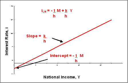
The LM curve will shift to the left (up) or right (down) whenever the intercept of the LM curve changes. Only a change in money supply, M, can cause the LM curve to shift.
| LM curve intercept = | - 1 • M < 0 h |
Because the intercept is a negative value an increase in money supply, M, will make the intercept more negative, which corresponds to a downward shift in the LM curve. A downward shift in the LM curve is the same thing as a rightward shift. An increase in the money supply causes the LM curve to shift to the right.
How much the LM curve shifts for a given change in money supply depends on the sensitivity of money demand to changes in the interest rate, or the value of the h coefficient. There are two possibilities, which we can describe in several equivalent ways:
| h is small | money demand is insensitive to changes in the interest rate money demand is interest inelastic it takes a large change in the interest rate to change money demand |
| h is large | money demand is very sensitive to changes in the interest rate money demand is interest elastic it takes only a small change in the interest rate to change money demand |
A change in money supply, M, shifts the LM curve. The size of the shift depends on the value of 1/h. If h is small, then 1/h is large and the shift in the LM curve will be large. If h is large, then 1/h will be small and the shift in the LM curve will be small. The larger the shift in the LM curve the greater effect a change in money supply may have on the economy.
One significant issue in the debate between the Keynesian and Classical economists has been over the response of money demand to changes in the interest rate. Keynes suggested that money demand was very interest elastic (h is large). In other words, an increase in money supply would be met immediately by an equal increase in money demand with no change in the interest rate. A change in money supply would have no effect on interest rates or the economy.
Classical economists, on the other hand, believed it would take an observable change in the interest rate to change money demand. Hence a change in money supply would be met with a large change in the interest rate, which would then impact investment spending and the economy.
The slope of the LM curve may be flat or steep again depending on how sensitive money demand is to change sin the interest rate (i.e., the value of h).
| LM curve slope = | k > 0 h |
The LM curve is steep (slope is a large positive number) when money demand is insensitive to changes in interest rate (h is small). For example, when the Federal Reserve Bank increases money supply a large change in the interest rate is needed to increase money demand to the new higher level of money supply. Changes to money supply have big impacts on interest rates. If a change in the interest rate significantly affects investment (and other) spending then changes in money supply can have big impacts on the economy.
The LM curve is flat (slope is close to zero) when only a small change in the interest rate leads to a large change in money demand (h is large). Essentially, the public is willing to hold whatever quantity of money is supplied. A change in money supply will have little impact on interest rates and the economy.
Note: we do not talk about the sensitivity of money demand to changes in income, k. This is because the relationship between money demand and income, while an important topic in economics, has not been the focus of debate between Keynesian and Classical economists.
In general, monetary policy is more effective (larger change in income for a given change in money supply) the steeper the LM curve and the greater the shift in the LM curve.
| Keynesian view | Classical view | |||
| Effect of change in money supply on national income | Small | Large | ||
| Is money demand sensitive to changes in the interest rate? | Very (h is large) | Somewhat (h is small) | ||
| Slope of LM curve | Flat (h is large) | Steep (h is small) | ||
| Shift of LM curve | Small (h is large) | Large (h is small) | ||
![]()
Equilibrium in the economy represents values of income and interest rate that simultaneously clear the goods and money markets. In other words, equilibrium occurs where the IS and LM curves intersect.
To determine the equilibrium national income in an economy set the IS equation solution for the interest rate (equation 2) equal to the LM equation solution for interest rate (equation 5), and solve for national income, Y.
| iIS = iLM | (6) |
Substituting equation (2) for iIS and equation (5) for iLM in equation (6) we have:
| 1 • (C0 + I0 + G0 - c • T0 + c • TR) - 1 - c(1-t) • Y b b |
= | - 1 • M + k • Y h h |
The solution to the model is some simple (but messy) algebra (see Appendix C for details of the calculation). Collect all the national income, Y, terms on one side and all other terms on the other side of the equation and solve for Y.
| Y = | b • M + h • (C0 + I0 + G0 - c • T0 + c • TR) h • [1 - c(1-t)] + b • k h • [1 - c(1-t)] + b • k |
To solve for the equilibrium interest rate you can substitute the equilibrium solution for income back into either the IS equation (2) or the LM equation (5).
In the previous sections on the IS and LM curves we only talked in general terms about how fiscal policy effectiveness relates to the sensitivity of investment to the interest rate (b) and how monetary policy effectiveness relates to the sensitivity of money demand to the interest rate (h). With the equilibrium solution to the IS-LM model we can be more specific about policy effectiveness because we can identify the fiscal and monetary policy "multipliers.".
Fiscal policy multiplier - how much does a change in government spending affect national income
| Fiscal policy multiplier = | h h • [1 - c(1-t)] + b • k |
Money supply multiplier - how much does change in money supply affect national income
| Monetary policy multiplier = | b h • [1 - c(1-t)] + b • k |
For Keynes, the coefficient h is large and b is small so that the fiscal policy multiplier reduces to 1/[1 - c(1-t)] (just like in the previous chapter) and the monetary policy multiplier = 0. For the Classical economists, h is small and b is large, so the fiscal policy multiplier = 0, and the monetary policy multiplier = 1/k.
![]()
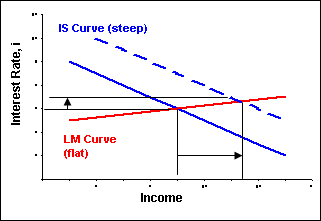
Expansionary fiscal policy represents an increase government spending or lower taxes. The objective of expansionary fiscal policy is to stimulate the economy and increase aggregate expenditures and national income. Expansionary fiscal policy causes the IS curve to shift to the right.
The economic effect of expansionary fiscal policy can be summarized as follows:
| Keynesian Case | Classical Case | |
 |
 | |
| Figure 6-5A. Keynesian Fiscal Policy | Figure 6-5B. Classical Fiscal Policy | |
| Flat LM curve - money demand is very sensitive to changes in the interest rate (h is large) - money demand can return to equilibrium with money supply only with a small increase in the interest rate. Essentially people are willing to hold as much money as is printed. | Steep LM curve - money demand is insensitive to changes in the interest rate (h is small) - money demand can return to equilibrium with money supply with only a large increase in the interest rate. | |
| Steep IS curve with large shift - investment spending is insensitive to changes in the interest rate (b is small) - large changes in the interest rate have little negative effect on investment spending. | Flat IS curve with small shift - investment spending is very sensitive to changes in the interest rate (b is large) - small changes in the interest rate can have a large negative effect on investment spending. |
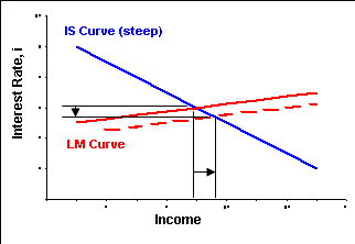
Expansionary monetary policy represents an increase the money supply. The objective of expansionary monetary policy is to stimulate the economy and increase aggregate expenditures and national income. Expansionary monetary policy causes the LM curve to shift to the right.
The economic effect of expansionary monetary policy can be summarized as:
| Keynesian Case | Classical Case | |
 |
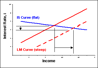 | |
| Figure 6-6A. Keynesian Monetary Policy | Figure 6-6B. Classical Monetary Policy | |
| Flat LM curve with small shift - money demand is very sensitive to changes in the interest rate (h is large) - money demand can return to equilibrium with money supply with only a small increase in the interest rate. | Steep LM curve with large shift - money demand is insensitive to changes in the interest rate (h is small) - money demand can return to equilibrium with money supply only with a large increase in the interest rate. | |
| Steep IS curve - investment spending is insensitive to changes in the interest rate (b is small) - large changes in the interest rate have little negative effect on investment spending. | Flat IS curve - investment spending is very sensitive to changes in the interest rate (b is large) - small changes in the interest rate can have a large negative effect on investment spending. |
One final word of caution. We make no mention of prices because we still maintain the Keynesian assumption of sticky prices. In other words, the average price level is unaffected by fiscal or monetary policy. While this is a very strong assumption it is not necessarily a theory killer. Since the end of the inflationary decade of the 1970s we have enjoyed a rather sustained period of relatively stable prices. For example, over the last 10 years the annual inflation rate has averaged 2.5 percent, ranging from a low of 1.6 percent in 1998 to 3.4 percent in 2000. This period includes years of strong economic growth as well as some of weak growth along with active fiscal and monetary policy. Nevertheless, we will try to develop a better understanding of the interaction of policy and prices over the next couple of chapters.
![]()
Given:
AE = C + I + G + NX
C = C0 + c • YD
I = I0 - b • i
G = G0
NX = 0
YD = Y - t • Y - T0 + TR
Step 1. Restate AE:
AE = C0 + c • YD + I0 - b • i + G0
= C0 + c • (Y - t • Y - T0 + TR) + I0 - b • i + G0
= C0 + c • Y - c • t • Y - c • T0 + c • TR + I0 - b • i + G0
= C0 + I0 + G0 - c • T0 + c • TR + c • (1 - t) • Y - b • i
Step 2. Apply goods market equilibrium condition:
Y = AE
Step 3. Substitute solution for AE from Step 1 into equilibrium condition in Step 2:
Y = C0 + I0 + G0 - c • T0 + c • TR + c • (1 - t) • Y - b • i
Step 4. IS curve - solve for i as function of Y. Carry the b • i term over to left-hand side and the Y on the left over to the right:
b • i = C0 + I0 + G0 - c • T0 + c • TR + c • (1 - t) • Y - Y
iIS = 1 • (C0 + I0 + G0 - c • T0 + c • TR) - 1 - c(1-t) • Y
b b
IS curve intercept = (1/b) • (C0 + I0 + G0 - c • T0 + c • TR) > 0
IS curve slope = - [1 - c(1-t)]/b < 0
Given:
Money demand: Md = k • Y - h • i
Money supply: Ms = M
Step 1. Apply money market equilibrium condition
Ms = Md
Step 2. Substitute for Ms and Md
M = k • Y - h • i
Step 3. LM curve - solve for i as function of Y:
iLM = - (1/h) • M + (k/h) • Y
LM curve intercept = - (1/h) • M < 0
LM curve slope = k/h > 0
iIS = iLM
| 1 • (C0 + I0 + G0 - c • T0 + c • TR) - 1 - c(1-t) • Y b b |
= | - 1 • M + k • Y h h |
Collect all Y terms on one side and all other terms on the other.
| 1 - c(1-t) • Y + k • Y b h |
= | 1 • M + 1 • (C0 + I0 + G0 - c • T0 + c • TR) h b |
Combine the Y terms:
| {h • [1 - c(1-t)] + b • k} • Y b • h |
= | 1 • M + 1 • (C0 + I0 + G0 - c • T0 + c • TR) h b |
What a mess -- solve for Y:
| Y = | b • M + h • (C0 + I0 + G0 - c • T0 + c • TR) h • [1 - c(1-t)] + b • k h • [1 - c(1-t)] + b • k |
File last modified: September 1, 2004
© Tancred Lidderdale (Tancred@Lidderdale.com)